Complex Numbers

A nonempty bounded subset of ZZ contains a maximal element

This assertion is used several times in these notes, here is its proof.

Let m be an arbitrary element of the set M in question, there is at least one, by assumption.
Further, let c be the bound. Then the algorithm

for n=c:-1:m do: if n ∈ M, break, fi, od

is guaranteed to halt after finitely many steps, and the current value of n is the maximal element
of M.

Also, note the corollary that a bounded function into the integers takes on its maximal value:
its range then contains a maximal element and any preimage of that maximal element will do.

Complex numbers

A complex number is of the form

z = a + ib.

with a and b real numbers, called, respectively, the real part of z and the imaginary part of z,
and i the imaginary unit, i.e.,



Actually, there are two complex numbers whose square is −1. We denote the other one by −i. Be
aware that, in parts of Engineering, the symbol j is used instead of i.

MATLAB works internally with (double precision) complex numbers. Both variables i
and j in MATLAB are initialized to the value i.

One adds complex numbers by adding separately their real and imaginary parts. One multiplies
two complex numbers by multiplying out and rearranging, mindful of the fact that i² = −1. Thus,

(a + ib)(c + id) = ac + aid + bic − bd = (ac − bd) + i(ad + bc).

Note that both addition and multiplication of complex numbers is commutative. Further, the
product of z = a + ib with its complex conjugate



is the nonnegative number



and its (nonnegative) squareroot is called the absolute value or modulus of z and denoted by



For z ≠ 0, we have l z l ≠ 0, hence is a well-defined complex number. It
is the reciprocal of z since , of use for division by z. Note that, for any two complex
numbers z and ,



It is very useful to visualize complex numbers as points in the so called complex plane, i.e.,
to identify the complex number a + ib with the point (a, b) in IR². With this identification, its
absolute value corresponds to the (Euclidean) distance of the corresponding point from the origin.

The sum of two complex numbers corresponds to the vector sum of their corresponding points. The
product of two complex numbers is most easily visualized in terms of the polar form



with r ≥ 0, hence r = l z l its modulus, and ∈ IR is called its argument. Indeed, for any real ,
has absolute value 1, and is the angle (in radians) that the vector
(a, b) makes with the positive real axis. Note that, for z ≠ 0, the argument, , is only defined up to
a multiple of 2π , while, for z = 0, the argument is arbitrary. If now also ,
then, by the law of exponents,



Thus, as already noted, the absolute value of the product is the product of the absolute values of
the factors, while the argument of a product is the sum of the arguments of the factors.

For example, in as much as the argument of is the negative of the argument of z, the argument
of the product is necessarily 0. As another example, if z = a + ib is of modulus 1, then z lies
on the unit circle in the complex plane, and so does any power z^k of z. In fact, then
for some real number , and therefore . Hence, the sequence , appears
as a sequence of points on the unit circle, equally spaced around that circle, never accumulating
anywhere unless = 0, i.e., unless z = 1.

(17.1) Lemma: Let z be a complex number of modulus 1. Then the sequence of powers of z lies on the unit circle, but fails to converge except when z = 1.

Convergence of a scalar sequence

A subset Z of C is said to be bounded if it lies in some ball



of ( finite) radius r. Equivalently, Z is bounded if, for some r, < r for all ∈ Z. In either case,
the number r is called a bound for Z.

In particular, we say that the scalar sequence is bounded if the set
is bounded. For example, the sequence (1, 2, 3, ...) is not bounded.

(17.2) Lemma: The sequence is bounded if and only if . Here, denotes the kth power of the scalar z.

Poof: Assume that > 1. I claim that, for all m,

(17.3)



This is certainly true for m = 1. Assume it correct for m = k. Then

The first term on the right-hand side gives



since > 1, while, for the second term, by induction hypothesis. Consequently,



showing that (17.3) also holds for m = k + 1.

In particular, for any given c, choosing m to be any natural number bigger than ,
we have . We conclude that the sequence is unbounded when > 1.
Assume that . Then, for any m, , hence the sequence
is not only bounded, it lies entirely in the unit disk



A sequence of (real or complex) scalars is said to converge to the scalar , in
symbols:



if, for all ε > 0, there is some so that, for all .

Assuming without loss the scalars to be complex, we can profitably visualize this definition as
saying the following: Whatever small circle of radius ε we draw around the
point , all the terms of the sequence except the first few are inside that circle.

Proof: If , then there is some so that, for all .
Therefore, for all m,



Note that r is indeed a well-defined nonnegative number, since a finite set of real numbers always
has a largest element.

(17.5) Lemma: The sequence is convergent if and only if either < 1 or else = 1. In the former case, , while in the latter case .

Proof: Since the sequence is not even bounded when > 1, it cannot be convergent in
that case. We already noted that it cannot be convergent when = 1 unless = 1, and in that
case for all m, hence also .

This leaves the case < 1. Then either = 0, in which case = 0 for all m, hence also
. Else, 0 < < 1, therefore is a well-defined complex number of modulus
greater than one, hence, as we showed earlier, grows monotonely to infinity as
m→∞. But this says that decreases monotonely to 0. In other words, .

Horner, or: How to divide a polynomial by a linear factor

Recall that, given the polynomial p and one of its roots, μ, the polynomial can
be constructed by synthetic division. This process is also known as nested multiplication or
Horner's scheme as it is used, more generally, to evaluate a polynomial efficiently. Here are the
details, for a polynomial of degree ≤ 3.

If , and z is any scalar, then

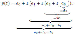
In other words, we write such a polynomial in nested form and then evaluate from the inside out.
Each step is of the form

"horner (17.6)

it involves one multiplication and one addition. The last number calculated is , it is the value
of p at z. There are 3 such steps for our cubic polynomial (the definition requires no
calculation!). So, for a polynomial of degree n, we would use n multiplications and n additions.

Now, not only is of interest, since it equals p(z), the other are also useful since



We verify this by multiplying out and rearranging terms according to powers of t. This gives

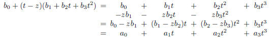
The last equality holds since, by (17.6),



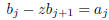
for j < 3 while by definition.

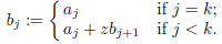
(17.7) Nested Multiplication (aka Horner): To evaluate the polynomial at the point z, compute the sequence   by the prescription Then , with In particular, if z is a root of p (hence = 0), then q(t) = p(t)/(t − z).

Since p(t) = (t − z)q(t), it follows that degq < deg p. This provides another proof (see (3.21))
for the easy part of the Fundamental Theorem of Algebra, namely that a polynomial of degree k
has at most k roots.