Classification and Linear Equations

Example. Find the general solution to

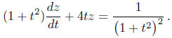
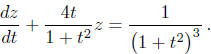
Solution. First bring the equation into the normal form

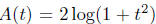
An integrating factor is where A′(t) = 4t/(1 + t²). Setting , we
see that

We then bring the differential equation into the integrating factor form

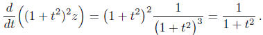
By integrating both sides of this equation we obtain

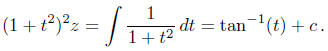
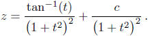
The general solution is therefore given by

2.3.2. Homogeneous Linear Equations. The linear equation (2.8) is said to be homogeneous
when r(t) = 0 for every t, and is said to be inhomogeneous otherwise. When (2.8) is
homogeneous its normal form (2.9) is simply

By formula (2.12) its general solution is simply

where A′(t) = a(t) and c is any constant . (2.14)

Hence, for homogenous linear equations the recipe for solution only requires finding one
primitive — namely, a primitive of a(t). This means that for simply enough a(t) you
should be able to write down general solutions immediately.

Example. Find the general solution to

Solution. Because a(t) = −5, a general solution is given by

, where c is an arbitrary constant .

Example. Find the general solution to

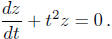
Solution. Because a(t) = t², a general solution is given by

where c is an arbitrary constant .

2.3.3. Initial-Value Problems for Linear Equations. In order to pick a unique solution
from the family (2.12) one must impose an additional condition that determines c. We do
this by again imposing an initial condition of the form

where is called the initial time and is called the initial value or initial datum. The
combination of the differential equation (2.9) with the above initial condition is

This is a so-called an initial-value problem. By imposing the initial condition upon the
family (2.12) we see that

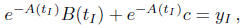
which implies that 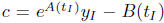. Therefore, if the primitives A(t) and B(t) exist
then the unique solution of initial-value problem (2.15) is given by

2.3.4. Existence of Solutions for Linear Equations. Even when you cannot find primitives
A(t) and B(t) analytically, you can show that a solution exists by appealing to the Second
Fundamental Theorem of Calculus whenever a(t) and f(t) are continuous over an interval
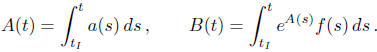
that contains the initial time . In that case one can express A(t) and B(t) as
the definite integrals

For this choice of A(t) and B(t) one has 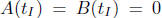, whereby formula (2.16)
becomes

The First Fundamental Theorem of Calculus implies that

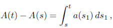
whereby formula (2.17) can be expressed as

This shows that if a and f are continuous over an interval that contains then the
initial-value problem (2.15) has a unique solution over , which is given by formula
(2.18).

For linear equations one can usually identify the interval of existence for the solution
of the initial-value problem (2.15) by simply looking at a(t) and f(t). Specifically, if Y (t) is
the solution of the initial value problem (2.15) then its interval of existence will be
whenever:

• the coefficient a(t) and forcing f(t) are continuous over ,
• the initial time is in ,
• either the coefficient a(t) or the forcing f(t) is not defined at both and .

This is because the first two bullets along with the formula (2.18) imply that the interval
of existence will be at least , while the last two bullets along with our definition
(2.2) of solution imply that the interval of existence can be no bigger than because
the equation breaks down at and . This argument works when or
.

Example: Give the interval of existence for the solution of the initial-value problem

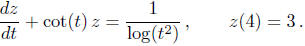
Solution: The coefficient cot(t) is not defined at t = nπ where n is any integer, and is
continuous everywhere else. The forcing 1/ log(t²) is not defined at t = 0 and t = 1, and
is continuous everywhere else. The interval of existence is therefore ( π, 2π ) because: both
cot(t) and 1/ log(t²) are continuous over this interval; the initial time is t = 4, which is in
this interval; cot(t) is not defined at t =π and t = 2π .

Example: Give the interval of existence for the solution of the initial-value problem

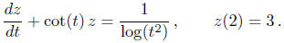
Solution: The interval of existence is (1,π) because: both cot(t) and 1/ log(t²) are con-
tinuous over this interval; the initial time is t = 2, which is in this interval; cot(t) is not
defined at t =π while 1/ log(t²) is not defined at t = 1.

Remark: If y = Y (t) is a solution of (2.15) whose interval of existence is then
this does not mean that Y (t) will become singular at either or when those
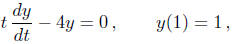
endpoints are finite. For example, y = t⁴ solves the initial-value problem

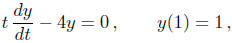
and is defined for every t. However, the interval of existence is just (0,∞) because the
initial time is t = 1 and normal form of the equation is

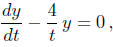
the coefficient of which is undefined at t = 0.

Remark: It is natural to ask why we do not extend our definition of solutions so that
y = t⁴ is considered a solution of the initial-value problem

for every t. For example, we might say that y = Y (t) is a solution provided it is differ-
entiable and satisfies the above equation rather than its normal form. However by this
definition the function

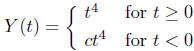
also solves the initial-value problem for any c. This shows that because the equation breaks
down at t = 0, there are many ways to extend the solution y = t⁴ to t < 0. We avoid such
complications by requiring the normal form of the equation to be defined.